Fem Pos Deviation Smoother
代码来源:Apollo 6.0分支 github
配置文件
先看下平滑器的配置文件,
位置:/apollo/modules/planning/conf/discrete_points_smoother_config.txt
内容: 1
2
3
4
5
6
7
8
9
10
11
12
13
14
15
16
17
18
19
20
21
22
23max_constraint_interval : 0.25
longitudinal_boundary_bound : 2.0
max_lateral_boundary_bound : 0.5
min_lateral_boundary_bound : 0.1
curb_shift : 0.2
lateral_buffer : 0.2
discrete_points {
smoothing_method: FEM_POS_DEVIATION_SMOOTHING
fem_pos_deviation_smoothing {
weight_fem_pos_deviation: 1e10
weight_ref_deviation: 1.0
weight_path_length: 1.0
apply_curvature_constraint: false
max_iter: 500
time_limit: 0.0
verbose: false
scaled_termination: true
warm_start: true
}
}
在ReferenceLineProvider的构造函数中,有选择平滑器的相关代码:
1 | if (smoother_config_.has_qp_spline()) { |
问题
参考modules/planning/math/discretized_points_smoothing/fem_pos_deviation_smoother.h代码中的注释: 1
2
3
4
5
6
7
8
9
10
11
12
13
14
15/*
* @brief:
* This class solve an optimization problem:
* Y
* |
* | P(x1, y1) P(x2, y2)
* | P(x0, y0) ... P(x(k-1), y(k-1))
* |P(start)
* |
* |________________________________________________________ X
*
*
* Given an initial set of points from 0 to k-1, The goal is to find a set of
* points which makes the line P(start), P0, P(1) ... P(k-1) "smooth".
*/
#### 原理
原理和公式可以参考这篇讲解,非常详细:https://zhuanlan.zhihu.com/p/342740447
Three quadratic penalties are involved:
- Penalty x on distance between middle point and point by finite element estimate;
- Penalty y on path length;
- Penalty z on difference between points and reference points
costX : \(\sum ((p_1 + p_3) - 2*p_2)^2\)
costY : \(\sum (p_{n+1} - p_n)^2\)
costZ : \(\sum (p_n - p_{refn})^2\)
General formulation of P matrix is as below(with 6 points as an example): I is a two by two identity matrix, X, Y, Z represents x * I, y * I, z * I 0 is a two by two zero matrix
\[\begin{vmatrix} X+Y+Z&-2X-Y&X&0&0&0\\ 0&5X+2Y+Z&-4X-Y&X&0&0\\ 0&0&6X+2Y+Z&-4X-Y&X&0\\ 0&0&0&6X+2Y+4Z&-4X-Y&X\\ 0&0&0&0&5X+2Y+Z&-2X-Y\\ 0&0&0&0&0&X+Y+Z\\ \end{vmatrix}\]
Only upper triangle needs to be filled
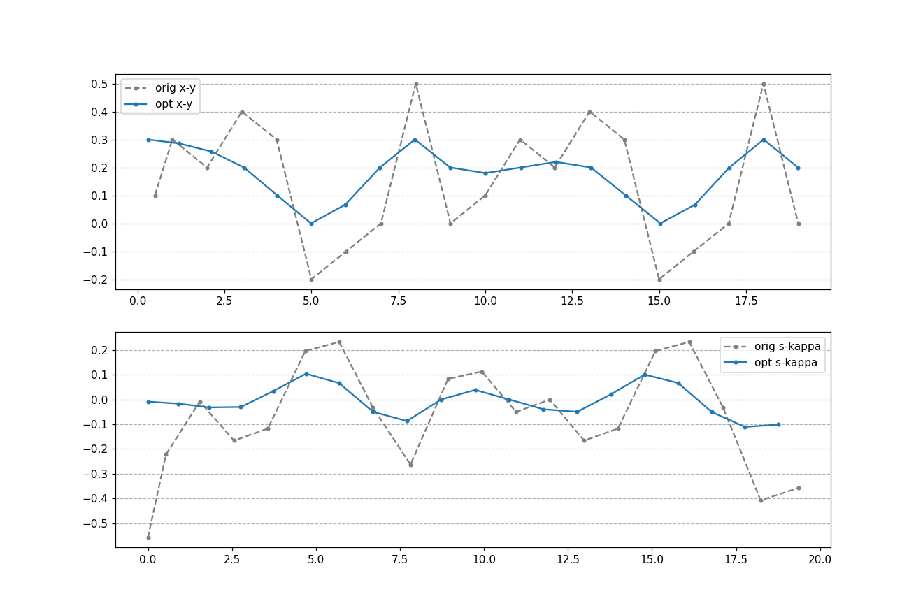
| #### 示例代码 用10个点模拟测试一下效果: | ||
|
||
| 查看结果: | ||
 |
||
| 上图灰线为原曲线,蓝色为平滑后的曲线 | ||
| 下图灰线为原曲线kappa,蓝线为平滑后的kappa | ||
| 可以看出平滑效果还不错。 |
使用测试数据再跑一下:
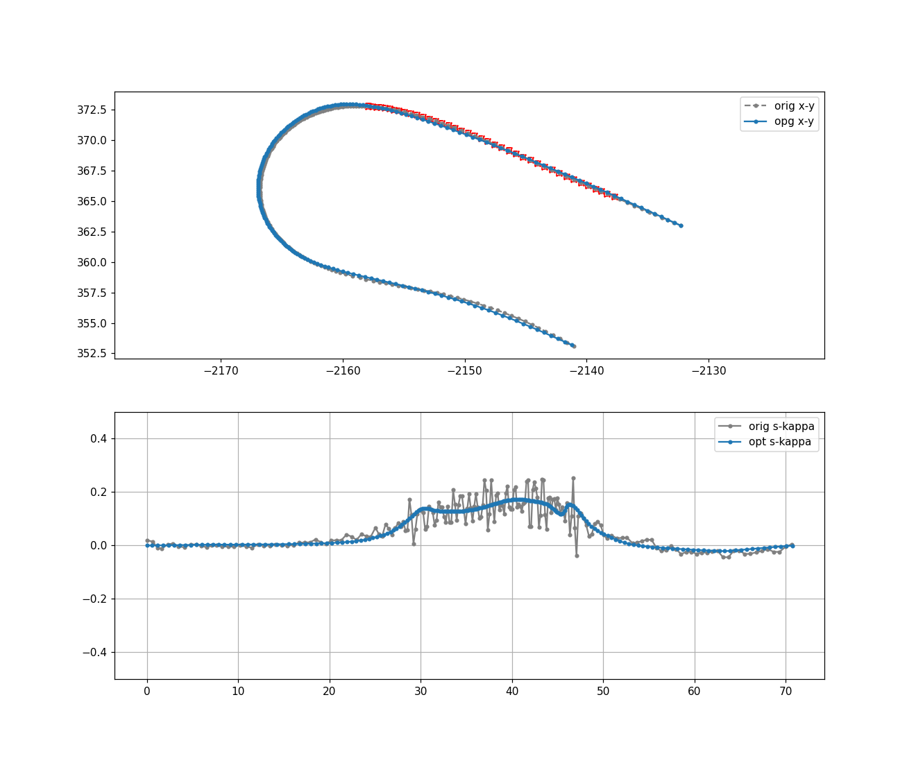
平滑前后的kappa对比非常明显
将bound也画出来:
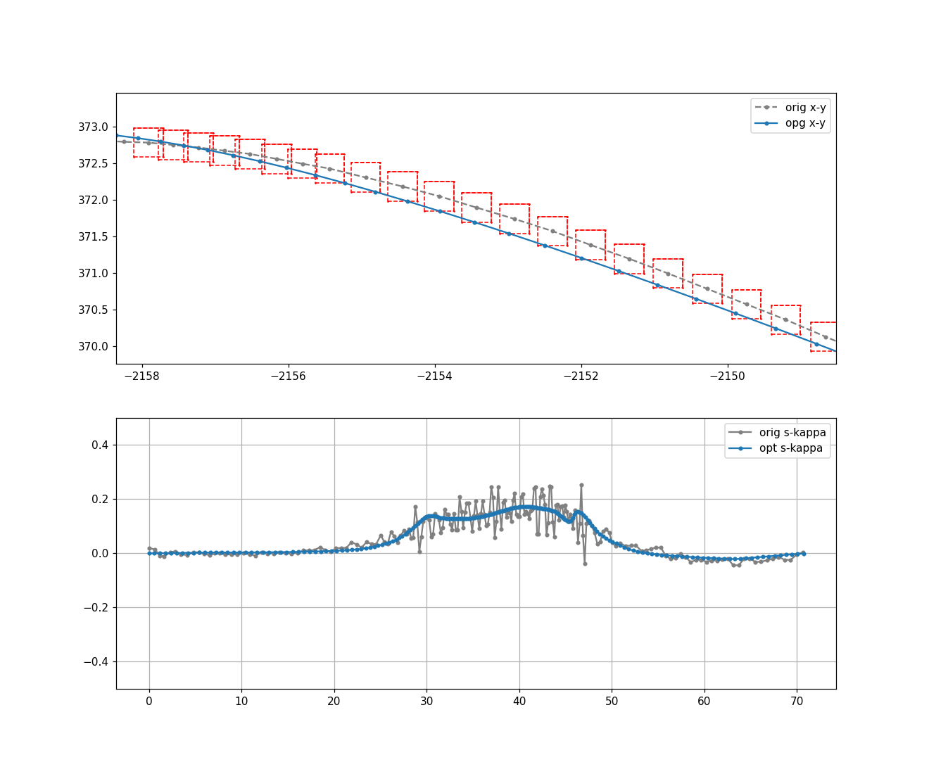
原曲线上的每个点,都生成一个矩形。
在该矩形中迭代求解使cost最小的点。